摘要

Cats vs. Dogs（猫狗大战）是Kaggle大数据竞赛某一年的一道赛题，利用给定的数据集，用算法实现猫和狗的识别。本博客设计了一个简单的两层卷积神经网络，利用TensorFlow深度学习框架进行模型训练，最终得到一个简单的二分类器。
本博客从数据集开始讲起，然后通过模型搭建、模型训练和模型测试依次讲解深度学习目标检测常用的步骤，并穿插着TensorFlow框架的基础知识讲解，语言通俗易懂，十分适合刚入门的初学者学习。

平台

系统：Windows 10
环境：python 3.5.4
编译器：Visual Studio Code

数据集处理

获取数据集

我们可以使用Kaggle官网上提供的数据集，读者可以在GitHub上下载，网址，或者从百度云下载：data，提取码：z9kn。当然了，我们也可以自己拍摄或采集一些数据集，为了保持和官网数据集命名格式的一致性，可以使用python的os库对自己采集的数据集进行批量重命名(如果是用官网的数据集，可以先跳过这一部分)。

import os


def rename_files(dir_path):
    """
    批量重命名文件
    参数：
        dirPath：文件路径
    """
    file_list = os.listdir(dir_path)

    index = 0
    for item in file_list:
        oldname = dir_path + r"\\" + file_list[index]
        newname = dir_path + r"\\" + "dog." + str(index) + ".jpg"
        os.rename(oldname, newname)

        index += 1

首先利用os.listdir()从文件夹中获取所有的文件名，返回值file_list依次存放着每个文件的名字。然后利用for循环依次遍历列表，最后利用os.rename()对其重命名。(如果需要重命名猫的照片，将dog替换成cat即可。)

1
2
3

if __name__ == "__main__":
    image_dir = r"D:\\TensorFlow\\dog_and_cat\\test"
    renameFiles(image_dir)

例如我在D:\\TensorFlow\\dog_and_cat\\test文件夹中存放着采集的数据集，调用rename_files()函数后，可以看到所有的文件名字已经全部重命名。

打乱数据集

为了提高数据集的鲁棒性和防止采集数据时的人为性，我们可以先将数据集随机打乱，至于是读取数据时还是训练时打乱，读者可以自己选择。本博客采用读取数据时打乱。

def get_all_files(file_path, is_random=True):
    """
    获取图片路径及其标签
    参数：
        file_path: a string 图片所在目录
        file_path：true or flase 是否乱序
    返回值：
        imageList：a list 图像列表
        lableList：a list 标签列表
    """
    image_list, label_list = [], []
    cat_count, dog_count = 0, 0

    # 从文件夹中读取文件名字
    for item in os.listdir(file_path):
        # listdir()：返回指定路径下的文件和文件夹列表
        item_path = file_path + '\\' + item
        item_label = item.split('.')[0]

        if os.path.isfile(item_path):
            # isfile()：判断某一路径是否为文件
            image_list.append(item_path)
        else:
            raise ValueError('no file.')

        if item_label == 'cat':
            label_list.append(0)
            cat_count += 1
        else:
            label_list.append(1)
            dog_count += 1

    print("There are %d cats, %d dogs." % (cat_count, dog_count))

    image_list = np.asarray(image_list)  # 当数据源是ndarray时，array会copy出一个副本，占用新的内存，但asarray不会
    label_list = np.asarray(label_list)

    if is_random:
        rnd_index = np.arange(len(image_list))
        np.random.shuffle(rnd_index)
        # 将文件乱序 # shuffle()：将序列的所有元素随机排序
        image_list = image_list[rnd_index]
        label_list = label_list[rnd_index]

    return image_list, label_list

首先初始化存储数据和标签的列表，然后依次遍历文件夹并读取名字，如果是文件则将文件名存储到image_list列表中，并将文件名的第一个参数存储到label_list列表中，然后分别统计猫和狗的数量。最后我们利用numpy中的shuffle()函数将列表打乱。

if __name__ == "__main__":
    image_dir = r"D:\\TensorFlow\\dogAndCat\\test"
    train_list = get_all_files(image_dir)
    print(train_list)

这里我们采用10张猫和10张狗的照片进行了一个简单的测试，其结果如图所示：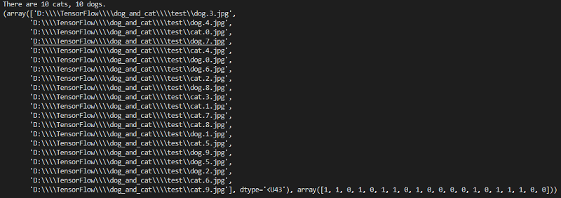
打乱数据集
可以看出所有的数据集都已经全部打乱。

数据集分批次处理

这里的处理主要涉及到两个方面，第一，分批次获取数据集，因为一次性将所有25000张图片载入内存不现实也不必要，所以将图片分成不同批次进行训练，第二，由于采集的数据集大小并不统一，所以很有必要先将其调整到一个统一的大小。
在讲解如何分批处理前，首先要知道TensorFlow是如何读取数据的。

tensorflow读取数据机制

TensorFlow中为了充分利用GPU，减少GPU等待数据的空闲时间，使用了两个线程分别执行数据读入和数据计算。具体来说就是使用一个线程源源不断的将硬盘中的图片数据读入到一个内存队列中，另一个线程负责计算任务，所需数据直接从内存队列中获取。
TensorFlow在内存队列之前，还设立了一个文件名队列，文件名队列存放的是参与训练的文件名，要训练N个epoch(1个epoch等于使用训练集中的全部样本训练一次)，则文件名队列中就含有N个批次的所有文件名。如图所示：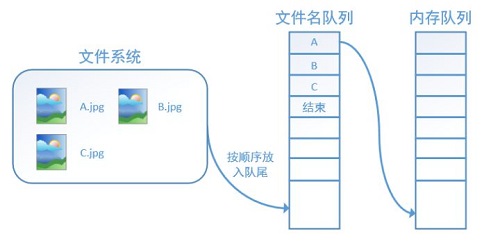
读取图片机制
在N个epoch的文件名最后是一个结束标志，当TensorFlow读到这个结束标志的时候，会抛出一个OutofRange 的异常，外部捕获到这个异常之后就可以结束程序了。
而创建TensorFlow的文件名队列就需要使用到 tf.train.slice_input_producer()函数。

tf.train.slice_input_producer()

tf.train.slice_input_producer()是一个tensor生成器，作用是按照设定，每次从一个tensor列表中按顺序或者随机抽取出一个tensor放入文件名队列。
其函数头为：

1	slice_input_producer(tensor_list, num_epochs=None, shuffle=True, seed=None, capacity=32, shared_name=None, name=None)

tensor_list是输入，格式为tensor的列表；一般为[data, label]，即由特征和标签组成的数据集，num_epochs是抽取batch(批次)的次数，如果没有给定值，那么将会抽取无数次batch(这会导致你训练过程停不下来)，如果给定值，那么在到达次数之后就会报OutOfRange的错误，shuffle是是否随机打乱，seed是随机种子，capcity是队列容量的大小，为整数，name是名称。
其返回值为tensor的列表，其结果和tensor_list一致。例如将之前的train_list作为输入，其结果显示为：

if __name__ == "__main__":
    image_dir = r"D:\\TensorFlow\\dog_and_cat\\test"
    train_list = get_all_files(image_dir, is_random=False)
    intput_queue = tf.train.slice_input_producer(train_list, shuffle=False)
    print(intput_queue)

结果为：
[<tf.Tensor 'input_producer/GatherV2:0' shape=() dtype=string>, <tf.Tensor 'input_producer/GatherV2_1:0' shape=() dtype=int32>]，其中第一个就是对应的image_list的向量，第二个为label_list。
有了队列之后就可以使用tf.train.batch()或tf.train.shuffle_batch()来生成批次大小为batch_size的tensor。

tf.train.batch()和tf.train.shuffle_batch()

其函数头为：

1	tf.train.batch([data, label], batch_size=batch_size, capacity=capacity,num_threads=num_thread,allow_smaller_final_batch=True)

1	tf.train.shuffle_batch([data, label], batch_size=batch_size, capacity=capacity,num_threads=num_thread,allow_smaller_final_batch=True)

[data，label]是输入的样本和标签，batch_size是batch的大小，capcity是队列的容量，num_threads是线程数，使用多少个线程来控制整个队列，allow_smaller_final_batch这个是当最后的几个样本不够组成一个batch的时候用的参数，如果为True则会重新组成一个batch。这2个区别在于一个是顺序产生，一个是随机产生(有shuffle是随机产生)。

batch取值

这里比较重要的一个参数是batch的取值，batch_size(批尺寸)是机器学习/深度学习中一个重要参数。其含义及取值可以参考这篇博客：网址
本博客采用的取值为batch_size=1，即每次只训练一个样本，也就是在线学习(Online Learning)。这也是Stochastic Gradient Descent(SGD，随机梯度下降算法)的更新规则，即：一次只进行一次更新，就没有冗余，而且比较快，并且可以新增样本。

生成数据集

def get_batch(train_list, image_size, batch_size, capacity, is_random=True):
    """
    分批次获取图片
    参数：
        train_list: 2-D list, [image_list, label_list]
        image_size: a int, 训练图像大小(image_size*image_size)
        batch_size: a int, 每个批次包含的样本数量
        capacity: a int, 队列容量
        is_random: True or False, 是否乱序
    返回值：
        image_train_batch：图像批次
        label_train_batch：标签批次
    """
    intput_queue = tf.train.slice_input_producer(train_list, shuffle=False)

    # 从路径中读取图片
    image_train = tf.read_file(intput_queue[0])
    image_train = tf.image.decode_jpeg(image_train, channels=3)  # 这里是jpg格式
    image_train = tf.image.resize_images(image_train, [image_size, image_size])
    image_train = tf.cast(image_train, tf.float32) / 255.  # 转换数据类型并归一化

    # 图片标签
    label_train = intput_queue[1]

    # 获取批次
    if is_random:
        image_train_batch, label_train_batch = tf.train.shuffle_batch([image_train, label_train],
                                                                      batch_size=batch_size,
                                                                      capacity=capacity,
                                                                      min_after_dequeue=100,
                                                                      num_threads=2)
    else:
        image_train_batch, label_train_batch = tf.train.batch([image_train, label_train],
                                                              batch_size=batch_size,
                                                              capacity=capacity,
                                                              num_threads=1)
    return image_train_batch, label_train_batch

获取到图片队列后，首先用read_file()读取图片，然后按照图片格式进行解码。本博客中训练数据是jpg格式的，所以使用decode_jpeg()解码器，如果是其他格式，就要用其他解码器。注意decode出来的数据类型是uint8，之后模型卷积层里面conv2d()要求输入数据为float32类型，所以如果删掉标准化步骤之后，需要进行类型转换。最后还需要将图片裁剪成相同大小(img_W和img_H)。这里使用resize_images()对图像进行缩放，而不是裁剪，采用NEAREST_NEIGHBOR插值方法。标签队列比较简单，直接获取即可。然后在利用tf.train.batch()将其分批次处理。
同样的我们进行简单的测试：

if __name__ == "__main__":
    image_dir = r"D:\\TensorFlow\\dog_and_cat\\test"
    train_list = get_all_files(image_dir, is_random=False)
    image_train_batch, label_train_batch = get_batch(train_list, 256, 1, 200, False)
    print(image_train_batch, label_train_batch)

这里我们将batch_size设置为1，也就是一次取一张照片，其输出结果为：
Tensor("batch:0", shape=(1, 256, 256, 3), dtype=float32) Tensor("batch:1", shape=(1,), dtype=int32)。

数据集可视化

之前的叙述都只是搭建模型，下面我们可以启动TensorFlow会话将图片显示出来。这里需要使用tf.train.Coordinator()来创建一个线程管理器(协调器)对象。

if __name__ == "__main__":
    import matplotlib.pyplot as plt
    image_dir = r"D:\\TensorFlow\\dog_and_cat\\test"
    train_list = get_all_files(image_dir, is_random=False)
    print(train_list)
    image_train_batch, label_train_batch = get_batch(train_list, 250, 1, 250, False)

    sess = tf.Session()

    coord = tf.train.Coordinator()   # 创建一个线程管理器(协调器)对象
    threads = tf.train.start_queue_runners(sess=sess, coord=coord)   # 启动tensor的入队线程

    try:
        for step in range(10):
            if coord.should_stop():
                break

            image_batch, label_batch = sess.run([image_train_batch, label_train_batch])  # 返回列表的值
            if label_batch[0] == 0:
                label = 'Cat'
            else:
                label = 'Dog'          

            # 显示图片
            plt.imshow(image_batch[0])
            plt.title(label)
            plt.show()           

    except tf.errors.OutOfRangeError:
        print('Done.')
    finally:
        coord.request_stop()

    coord.join(threads=threads)
    sess.close()

在讲解这部分代码之前，我们首先要简单了解一下TensorFlow的多线程概念。
TensorFlow的Session对象是支持多线程的，可以在同一个会话(Session)中创建多个线程，并行执行。在Session中的所有线程都必须能被同步终止，异常必须能被正确捕获并报告，会话终止的时候，队列必须能被正确地关闭。
TensorFlow提供了两个类来实现对Session中多线程的管理：tf.Coordinator和tf.QueueRunner，这两个类往往一起使用。Coordinator类用来管理在Session中的多个线程，可以用来同时停止多个工作线程并且向那个在等待所有工作线程终止的程序报告异常，该线程捕获到这个异常之后就会终止所有线程。使用tf.train.Coordinator()来创建一个线程管理器(协调器)对象。
QueueRunner类用来启动tensor的入队线程，可以用来启动多个工作线程同时将多个tensor(训练数据)推送入文件名称队列中，具体执行函数是tf.train.start_queue_runners，只有调用 tf.train.start_queue_runners之后，才会真正把tensor推入内存序列中，供计算单元调用，否则会由于内存序列为空，数据流图会处于一直等待状态。

结合上述理论，我们再次了解一下TensorFlow的数据读取机制：
读取图片机制_2

调用 tf.train.slice_input_producer，从本地文件里抽取tensor，准备放入Filename Queue（文件名队列）中;
调用 tf.train.batch，从文件名队列中提取tensor，使用单个或多个线程，准备放入文件队列;
调用 tf.train.Coordinator() 来创建一个线程协调器，用来管理之后在Session中启动的所有线程;
调用tf.train.start_queue_runners, 启动入队线程，由多个或单个线程，按照设定规则，把文件读入Filename Queue中。函数返回线程ID的列表，一般情况下，系统有多少个核，就会启动多少个入队线程（入队具体使用多少个线程在tf.train.batch中定义）;
文件从 Filename Queue中读入内存队列的操作不用手动执行，由tf自动完成;
调用sess.run 来启动数据出列和执行计算;
使用 coord.should_stop()来查询是否应该终止所有线程，当文件队列（queue）中的所有文件都已经读取出列的时候，会抛出一个OutofRangeError 的异常，这时候就应该停止Sesson中的所有线程了;
使用coord.request_stop()来发出终止所有线程的命令，使用coord.join(threads)把线程加入主线程，等待threads结束。

有了上述2个理论基础，我们就可以理解之前的代码了，首先启动会话，然后启动线程管理器，然后将之前的训练数据依次放入队列中，这里加了一个图片显示，主要是利用matplotlib这个库，最后在依次终止所有的线程和会话。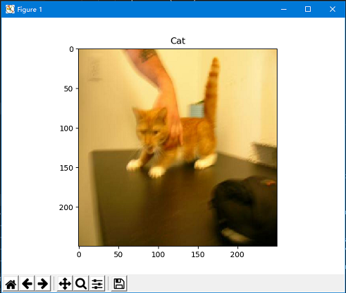
显示图片
这是其中的一张图片的显示结果。

模型搭建

有了数据集后，我们就可以正式搭建卷积神经网络的结构了。这里主要是仿照TensorFlow的官方例程cifar-10网络结构来写的。就是两个卷积层（每个卷积层后加一个池化层），两个全连接层，最后一个softmax输出分类结果。

import tensorflow as tf

def inference(images, batch_size, n_classes):
    # conv1, shape = [kernel_size, kernel_size, channels, kernel_numbers]
    with tf.variable_scope("conv1") as scope:
        weights = tf.get_variable("weights",
                                  shape=[3, 3, 3, 16],
                                  dtype=tf.float32,
                                  initializer=tf.truncated_normal_initializer(stddev=0.1, dtype=tf.float32))
        biases = tf.get_variable("biases",
                                 shape=[16],
                                 dtype=tf.float32,
                                 initializer=tf.constant_initializer(0.1))
        conv = tf.nn.conv2d(images, weights, strides=[1, 1, 1, 1], padding="SAME")
        pre_activation = tf.nn.bias_add(conv, biases)
        conv1 = tf.nn.relu(pre_activation, name="conv1")

    # pool1 && norm1
    with tf.variable_scope("pooling1_lrn") as scope:
        pool1 = tf.nn.max_pool(conv1, ksize=[1, 3, 3, 1], strides=[1, 2, 2, 1],
                               padding="SAME", name="pooling1")
        norm1 = tf.nn.lrn(pool1, depth_radius=4, bias=1.0, alpha=0.001/9.0,
                          beta=0.75, name='norm1')

    # conv2
    with tf.variable_scope("conv2") as scope:
        weights = tf.get_variable("weights",
                                  shape=[3, 3, 16, 16],
                                  dtype=tf.float32,
                                  initializer=tf.truncated_normal_initializer(stddev=0.1, dtype=tf.float32))
        biases = tf.get_variable("biases",
                                 shape=[16],
                                 dtype=tf.float32,
                                 initializer=tf.constant_initializer(0.1))
        conv = tf.nn.conv2d(norm1, weights, strides=[1, 1, 1, 1], padding="SAME")
        pre_activation = tf.nn.bias_add(conv, biases)
        conv2 = tf.nn.relu(pre_activation, name="conv2")

    # pool2 && norm2
    with tf.variable_scope("pooling2_lrn") as scope:
        pool2 = tf.nn.max_pool(conv2, ksize=[1, 3, 3, 1], strides=[1, 2, 2, 1],
                               padding="SAME", name="pooling2")
        norm2 = tf.nn.lrn(pool2, depth_radius=4, bias=1.0, alpha=0.001/9.0,
                          beta=0.75, name='norm2')

    # full-connect1
    with tf.variable_scope("fc1") as scope:
        reshape = tf.reshape(norm2, shape=[batch_size, -1])
        dim = reshape.get_shape()[1].value
        weights = tf.get_variable("weights",
                                  shape=[dim, 128],
                                  dtype=tf.float32,
                                  initializer=tf.truncated_normal_initializer(stddev=0.005, dtype=tf.float32))
        biases = tf.get_variable("biases",
                                 shape=[128],
                                 dtype=tf.float32,
                                 initializer=tf.constant_initializer(0.1))
        fc1 = tf.nn.relu(tf.matmul(reshape, weights) + biases, name="fc1")

    # full_connect2
    with tf.variable_scope("fc2") as scope:
        weights = tf.get_variable("weights",
                                  shape=[128, 128],
                                  dtype=tf.float32,
                                  initializer=tf.truncated_normal_initializer(stddev=0.005, dtype=tf.float32))
        biases = tf.get_variable("biases",
                                 shape=[128],
                                 dtype=tf.float32,
                                 initializer=tf.constant_initializer(0.1))
        fc2 = tf.nn.relu(tf.matmul(fc1, weights) + biases, name="fc2")

    # softmax
    with tf.variable_scope("softmax_linear") as scope:
        weights = tf.get_variable("weights",
                                  shape=[128, n_classes],
                                  dtype=tf.float32,
                                  initializer=tf.truncated_normal_initializer(stddev=0.005, dtype=tf.float32))
        biases = tf.get_variable("biases",
                                 shape=[n_classes],
                                 dtype=tf.float32,
                                 initializer=tf.constant_initializer(0.1))
        softmax_linear = tf.add(tf.matmul(fc2, weights), biases, name="softmax_linear")
        softmax_linear = tf.nn.softmax(softmax_linear)
    return softmax_linear

整体主要分为三个部分，即卷积+池化层，全连接层，softmax输出。
在正式讲解前，我们先了解几个比较重要的函数。

tf.nn.conv2d()：卷积函数
函数头为：tf.nn.conv2d(input, filter, strides, padding, use_cudnn_on_gpu=None, name=None)
input：输入图像，形式为：[batch, in_height, in_width, in_channels]，即训练一个batch的图片数量，图片高度，图片宽度，图像通道数。
filter：相当于卷积核，形式为：[filter_height, filter_width, in_channels, out_channels]，具体含义为：[卷积核的高度，滤波器的宽度，图像通道数，滤波器个数]，这里的第三维in_channels就是参数input的第四维。
strides：卷积时在图像每一维的步长，是一个一维的向量，长度为4，其中strides[0]=strides[3]=1，strides[1]表示输入图像in_height的滑动步长，strides[2]表示输入图像in_weight的滑动步长。
padding：当其值为VALID时，表示边缘不填充，当其值为SAME时，表示填充。
tf.nn.max_pool()：池化函数
函数头为：tf.nn.max_pool(input, ksize, strides, padding, name=None)
这里面的input,strides和padding和之前的卷积函数里面的几乎一样，唯一有点不同的是ksize，这个表示池化窗口的大小，一般是[1,height,width,1]，因为一般我们不在batch和channels上做池化，所以这两个维度都设为1。
tf.nn.lrn()：局部响应归一化函数
函数头为：tf.nn.lrn(input,depth_radius=None,bias=None,alpha=None,beta=None,name=None)
局部响应归一化原理是仿造生物学上活跃的神经元对相邻神经元的抑制现象(侧抑制)，其公式如下：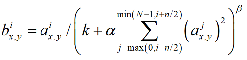

计算方法如下：
sqr_sum[a, b, c, d] = sum(input[a, b, c, d - depth_radius : d + depth_radius + 1] ** 2),output = input / (bias + alpha * sqr_sum) ** beta。
N表示通道数(channel)。a,n/2,k,α,β分别表示函数中的input,depth_radius,bias,alpha,beta。具体含义可以参考这篇博客：网址。

卷积+池化层

这里一共有2层，首先利用tf.variable_scope()定义变量的作用域并重命名，下同。然后利用tf.get_variable()分别创建weights变量和biases变量，下同。truncated_normal_initializer()和tf.constant_initializer()都是参数初始化函数，读者可以自己查阅。然后利用tf.nn.conv2d()函数进行卷积，其中input为图像，也就是函数的输入，filter为weights，这里的取值为[3,3,3,16]，前面的2个3表示滤波器的大小为3*3，后面的3是因为图像的通道数为3，最后的16表示一共使用16个3*3的滤波器。stride取值为1，即步长为1，且边缘填充。最后将其和偏差相加并输入到Rule激活函数中，下同。
接下来就是一个池化层，相比较卷积层要简单了很多，这里的input就是刚才的池化层1，即conv1，ksize取值为[1,3,3,1]，即滤波器的大小为3*3，这里的stride取值为2，且边缘填充。最后使用tf.nn.lrn()进行局部响应归一化。
第二个的卷积和池化层和第一个类似，这里就不再叙述了。值得注意的是第二个卷积层中的[3,3,16,16]里面的第1个16表示的是上一层卷积层的第四个维度16，即16个滤波器的16。

全连接层

全连接层是将所有的元素平整化为一个一维向量。每个全连接层的权重长度为2，分别为上一层的长度和该层的长度，从代码可以看出，两个全连接层的长度都是128，其中第一个全连接层的上一层长度是根据之前的池化层算出来的，也就是将所有的特征图的参数相乘，具体见下文分析。

softmax

最后一个是softmax层，也就是最后的分类输出，其最后的网络输出长度也就是分类的个数，也就是函数的输入n_classes。

损失函数及评估

搭建好网络结构后，后面的损失函数及评估就十分简单了，这里使用的是交叉熵损失函数，tf.nn.in_top_k()的使用方法也比较简单，读者可以自己查阅。

def losses(logits, labels):
    with tf.variable_scope('loss'):
        cross_entropy = tf.nn.sparse_softmax_cross_entropy_with_logits(logits=logits,
                                                                       labels=labels)
        loss = tf.reduce_mean(cross_entropy)
    return loss


def evaluation(logits, labels):
    with tf.variable_scope("accuracy"):
        correct = tf.nn.in_top_k(logits, labels, 1)
        correct = tf.cast(correct, tf.float16)
        accuracy = tf.reduce_mean(correct)
    return accuracy

网络结构再分析

我们以208*208*3的输入图像为例，将卷积网络结构的形状、大小及参数汇总到如下的表格中：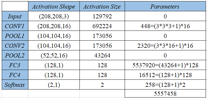
参数统计
表中的第一列为每一层维度大小，第一个卷积层的16也就是该层使用的滤波器个数，而池化层会将之前的维度减半，后面的全连接层是一个一维列向量。表中的第二列为每一层的激活值尺寸，即将之前的维度全部相乘得到的值，第三列是每一层的参数个数。卷积层的计算公式为：(滤波器参数+1)*滤波器个数，其中1表示偏差。池化层没有参数，全连接层的计算公式为：(上一层维度+1)*这一层维度，这里的1也表示偏差。
我们也可以用TensorFlow里面的tf.trainable_variables()将训练的变量找到并计算其数量：

if __name__ == '__main__':
    image_dir = r'D:\\TensorFlow\\dog_and_cat\\data\\train'

    sess = tf.Session()

    train_list = get_all_files(image_dir, True)
    image_train_batch, label_train_batch = get_batch(train_list, 208, 8, 200, True)
    train_logits = inference(image_train_batch, 2)

    var_list = tf.trainable_variables()
    for v in var_list:
        print(v, end='\n')
    paras_count = tf.reduce_sum([tf.reduce_prod(v.shape) for v in var_list])
    print('The number of parameters are :%d' % sess.run(paras_count), end='\n\n')

结果显示为：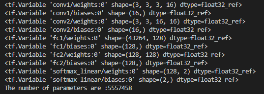
参数统计_代码
可以看出，其结果和之前我们计算的一致。
注：paras_count计算步骤为：先找到每个变量的维度，然后再计算各个维度相乘的积，最后再求和。
由表可见，随着卷积网络的加深，激活值尺寸由开始的692224，慢慢地减少到43264，最后减少到softmax层的2，当然如果激活尺寸下降太快，也会影响神经网络的性能。我们还能观察到其大部分的参数都是集中在全连接层。
当然了，这个卷积网络的参数也可以取其他的值。读者可以在代码中自行修改。

模型训练

下面就是将之前的函数综合起来进行模型训练。

import time
from load_data import *
from model import *
import matplotlib.pyplot as plt


# 训练模型
def training():
    N_CLASSES = 2
    IMG_SIZE = 208
    BATCH_SIZE = 8
    CAPACITY = 200
    MAX_STEP = 10000
    LEARNING_RATE = 1e-4

    # 测试图片读取
    image_dir = r'D:\\TensorFlow\\dog_and_cat\\data\\train_2'

    sess = tf.Session()

    train_list = get_all_files(image_dir, True)
    image_train_batch, label_train_batch = get_batch(train_list, IMG_SIZE, BATCH_SIZE, CAPACITY, True)
    train_logits = inference(image_train_batch, N_CLASSES)
    train_loss = losses(train_logits, label_train_batch)
    train_acc = evaluation(train_logits, label_train_batch)
    train_op = tf.train.AdamOptimizer(LEARNING_RATE).minimize(train_loss)

    saver = tf.train.Saver()

    sess.run(tf.global_variables_initializer())

    coord = tf.train.Coordinator()
    threads = tf.train.start_queue_runners(sess=sess, coord=coord)

    s_t = time.time()
    try:
        for step in range(MAX_STEP):
            if coord.should_stop():
                break

            _, loss, acc = sess.run([train_op, train_loss, train_acc])

            if step % 100 == 0:  # 实时记录训练过程并显示
                runtime = time.time() - s_t
                print('Step: %6d, loss: %.8f, accuracy: %.2f%%, time:%.2fs, time left: %.2fhours'
                      % (step, loss, acc * 100, runtime, (MAX_STEP - step) * runtime / 360000))
                s_t = time.time()

        saver.save(sess, r'D:\\TensorFlow\\dog_and_cat\\log\\model.cpkt')

    except tf.errors.OutOfRangeError:
        print('Done.')
    finally:
        coord.request_stop()

    coord.join(threads=threads)
    sess.close()

首先初始化一些参数，其中分类类别为2，图像大小为208*208，batch_size为8，即一次训练8张图片，容量为200，迭代次数为10000，学习率为1e-4。然后初始化图片存放的位置。
下面就正式启动会话，开始训练。先用get_all_files()函数将图片全部读入到train_list列表中，然后将该列表放到get_batch中获取训练批次image_train_batch和label_train_batch，其次放入到之前设计好的卷积网络模型中，得到模型的输出train_logits，并依次进行损失函数和评估处理以得到正确率。最后使用自适应矩估计算法AdamOptimizer()进行反向传播的参数优化。
接下来是用Saver()将训练好的模型保存，因为卷积网络的计算量很大，每次运行都耗费很长时间，所以很有必要将训练好的模型保存以便下次处理。
再往下就是调用run()函数实际运行了，首先初始化所有变量，然后调用线程(见上文分析)，最后就是迭代训练，每100次显示训练的正确率。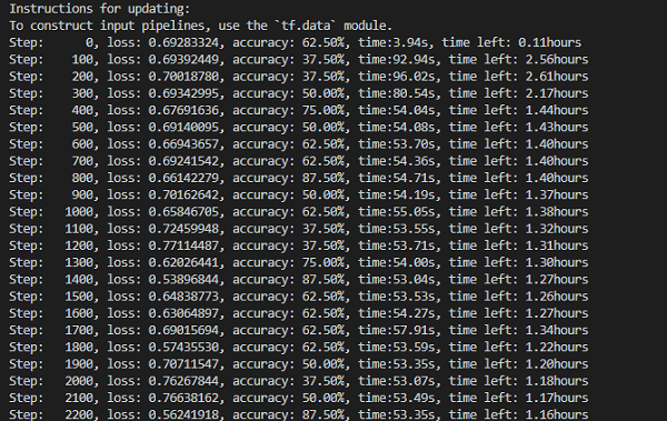
模型训练
注：如果设置迭代次数为10000次，一次训练大概需要2个小时左右。

模型测试

训练好模型后，就可以拿测试集数据来检验模型的正确性了。

def eval():
    N_CLASSES = 2
    IMG_SIZE = 208
    BATCH_SIZE = 1
    CAPACITY = 200
    MAX_STEP = 10

    test_dir = r'D:\\TensorFlow\\dog_and_cat\\data\\test'

    sess = tf.Session()

    train_list = get_all_files(test_dir, is_random=True)
    image_train_batch, label_train_batch = get_batch(train_list, IMG_SIZE, BATCH_SIZE, CAPACITY, True)
    train_logits = inference(image_train_batch, N_CLASSES)
    train_logits = tf.nn.softmax(train_logits)  # 用softmax转化为百分比数值

    # 载入模型
    saver = tf.train.Saver()
    saver.restore(sess, 'log\\model.cpkt')
    coord = tf.train.Coordinator()
    threads = tf.train.start_queue_runners(sess=sess, coord=coord)

    try:
        for step in range(MAX_STEP):
            if coord.should_stop():
                break

            image, prediction = sess.run([image_train_batch, train_logits])
            print('prediction', prediction)
            max_index = np.argmax(prediction)
            if max_index == 0:
                label = '%.2f%% is a cat.' % (prediction[0][0] * 100)
            else:
                label = '%.2f%% is a dog.' % (prediction[0][1] * 100)

            plt.imshow(image[0])
            plt.title(label)
            plt.show()

    except tf.errors.OutOfRangeError:
        print('Done.')
    finally:
        coord.request_stop()

    coord.join(threads=threads)
    sess.close()

程序和训练模型的程序几乎一致，唯一的区别在于，这里放入run()函数运行的部分是image_train_batch和train_logits，即图像批次和训练结果。这里的prediction也就是每个类别的置信度，即是猫或是狗的概率。接下来就是分析该概率，接近于0则表示是猫，否则为狗。最后用matplotlib库将图像显示出来：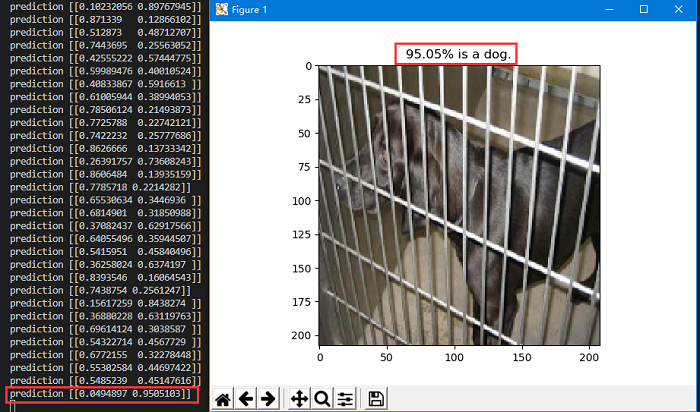
测试结果
这是某一张图的结果，从结果可以看出，该模型的输出结果为[0.0494897,0.9505103]，即认为4%的概率是猫，95%的概率是狗。

结论

本博客利用TensorFlow搭建了一个简单的两层卷积神经网络结构，基本实现了猫狗分类器，正确率和置信度总体上还可以，基本上能达到要求，毕竟我们只是使用了一个非常简单的卷积网络，但正确率和置信度仍有提高的空间，读者可以适当的增加网络层数，并设置好相应的参数，以改变模型的正确率。
由于本人也是初学深度学习，有写的不好或写错的地方还望读者多多留言指出，以便后续的改进。